notes

The Analytics Edge

Instructors - Bikramjit Das, Stefano Galelli

The Analytics Edge
- Course Overview
- Course timetable
General procedures
Basics of R
Preprocessing
Data visualization
- Assorted plots
- Scatter plots
Result analysis
Predictive Models I
Predictive Models II
Non-predictive models

Course Overview

Grading Component	Weightage (%)
Mid-Term Test (Week 6)	30
Competition (Week 13)	38
Final Test (Week 14)	30
Course Feedback Completion	2

Course timetable

Week	Description
1	Introduction to Analytics and the Software R with Visualization. Recall: Statistical tests, tools.
2	Method: Linear Regression Predicting the quality and prices of wine (Wine analytics) Moneyball (Sports analytics)
3	Method: Logistic Regression Predicting the failure of space shuttles (Challenger) Predicting the risk of coronary heart disease (Framingham Heart Study)
4	Method: Multinomial Logit and Mixed Logit in Discrete Choice Predicting the Academy Award winners (Oscars) Estimating the preference for safety features in cars
5	Methods: Big Data and Analytics: Model Selection Baseball (Sports) Cross-country growth regressions (Economics)
6	Review and Test (23 October, Wednesday, 2-4 pm)
7	Break
8	Method: Classification and Regression Trees (CART), Random Forests Forecasting Supreme Court Decisions (Law)
9	Method: Logistic Regression, CART, Random Forests in Text Analytics Twitter (Social media), Enron (Email)
10	Method: Clustering, Collaborative and Content Filtering Netflix, MovieLens (Recommendation systems)
11	Method: Singular Value Decomposition, Censored Data Photos, Netflix, Redbook (Marital), Stanford Heart Transplant (Healthcare)
12	Method: Optimization Revenue Management, Capstone Allocation
13	Review and Competition
14	Test

General procedures

Pre-flight checklist

Make sure you can import these libraries in R notebook.

library(ggplot2)
library(psych)
library(ggfortify)
library(leaps)
library(caTools)
library(mlogit)
library(zoo)
library(glmnet)
library(rpart)
library(rpart.plot)
library(tm)
library(randomForest)
library(SnowballC)
library(wordcloud)
library(e1071) # Naive Bayes
library(jpeg)
library(survival)
library(flexclust) # for finals
library(caret)

rm(list=ls())

If you cannot, please panic.

Common errors

Please remember the . when you are training against the rest of the data. responsive~.,

GLM requires you to put family='binomial'

Do not train on the test data. Please copy correctly.

Adjusted R-squared is not R-squared, please ask the examiners.

Helper functions

To understand a function, use ? to read the offline documentation. To understand an object, use attributes(x) to see the attributes.

For MacOS Refer to the the ‘Run’ option on the top right of this window to see the shortcut related to running and restarting the cell.

Run line Cmd + Enter
Run chunk Shift + Cmd + Enter
Run all Opt + Cmd + R
New R Cell Cmd + Opt + I
Comment Cmd + / (custom)

Header to specify html-knitting output and remove environment variables

---
output:
  html_document: default
---

rm(list=ls())

Introduction to statistics

R-squared - higher better Adjusted R-squared - higher better **AIC - lower better ** Likelihood - higher better Loglikehilood - higher better Negative loglikelihood (logloss?) - lower better KL divergence - zero the same, higher more different

Basics of R

A dataframe is not a matrix. A dataframe may have named or unnamed columns. A vector is not a column. Can a vector have named values? Can a matrix have named values?

Common functions

names()
apply()
# (X, MARGIN, FUN), MARGIN = row or columns
tapply()
# data(iris); tapply(iris$Sepal.Width, iris$Species, median)
unname()
unique()
paste0()
which()
subset() 
coef() # extract coefficient from linear models

Numerical functions

sum(arr)
prod(arr)
exp(arr)
var(arr)
sd(arr)
summary(arr)
which.max(arr)
pmax(arr,arz)  # take maximum element-wise
arr > 3  # you can implement element-wise logical check

# colMeans() # calculate the mean of each column?
cor(matrix[,COL_S:COL_E])

is.na() # counts number of NA
mean() # R has this function, ignores NA values

Type casting

z <- c(0:9)
class(z)  # prints class
as.numeric(z)  # casts into float?

z1 <- c("a","b","d")
w <- as.character(z1)
as.integer(w)  # returns array of NA

as.factor(w)  # required for classification models

Matrices

The matrix operations may require some explanation.

definition x<-matrix(c(3,-1,2,-1),nrow=2, ncol=2)
e-wise multiplication x*x, x*2
matrix multiplication x%*%x
transpose t(x)
read element r[2,2], r[3], starts counting from one
inverse of a matrix (?) solve(x)
solving system of linear equations a%*%solve(a)
get eigenvectors eigen(a)$vectors

Dataframes

You are unlikely to do this, you are likely to load csv files.

CELG <- data.frame(names=c("barack","serena"),
                   ages=c(58,38),
                   children=c(2,1))
# append to dataframe
CELG$spouse <- c("michelle","alexis")

# use negative signs to exclude columns or rows
test_2 <- df_2[-trainid_2,]

Statisitical testing

t.test(oscars$Nom[oscars$PP==1 & oscars$Ch==1],
       oscars$Nom[oscars$PP==1 & oscars$Ch==0],
       alternative = clib("greater"))

Miscellaneous

# date configuration
base::as.Date(32768, origin = "1900-01-01")

# to remove intercept, fit to -1
MPP2 <- mlogit(Ch~Nom+Dir+GG+PGA-1, data=D1)

Preprocessing

You need to preprocess the data.

Data reading

poll <- read.csv("AnonymityPoll.csv", stringsAsFactors=FALSE)
# consider stringsAsFactors
summary(poll)  # 7-figure summary of every column
str(poll)  # see some data

table(poll$Smartphone)  # freqency in a column
summary(poll$Smartphone)  # 7-figure summary of a column

# freqency matrix of two columns
table(poll$Internet.Use, poll$Smartphone)

# find the mean of the first value depending on second
tapply(limited$Info.On.Internet, 
       limited$Smartphone, 
       mean)

# count number of NA in a column
sum(is.na(poll$Internet.Use))

Data manipulation

# remove rows with any (?) NA variables
hitters = na.omit(hitters)

# obtain a subset
limited <- subset(poll, poll$Internet.Use == 1)

# obtain a subset without a column
eg1 <- subset(eg,select=-c(Country))

# obtain a subset with 'or' logic operator
limited <- subset(poll, poll$Internet.Use == 1|
                        poll$Smartphone == 1)

# row subset
# column subset

Combining dataframes

To combine dataframes one after another row, and fill empty cells.

library(plyr)
combined <- rbind.fill(train, test)

To combine dataframes beside one another and fill empty cells.

library(dplyr)
combined_features <- within(combined, rm(tweet, Id))

Train-test split

Please do it correctly and not lose two subgrades.

set.seed(144)
library(caTools)

# train-test split, stratified
split <- sample.split(framing1$TENCHD,SplitRatio=0.65)
training <- subset(framing1,split==TRUE)
test <- subset(framing1,split==FALSE)

SongsTrain <- subset(songs, songs$year<=2008)
SongsTest <- subset(songs, songs$year==2009 | songs$year==2010)

Cross validation

Week 5b

Simpler models often tend to work better for out-of-sample predictions and so we will penalize models for excessive model complexity.

With the increase in computational power, we can partition the data set into training, validation and test sets and conduct model assessment and selection.

The training set is used to estimate the model parameters.
The validation set is used to do model selection.
The test set is the evaluation set on which we will simply evaluate or check how the model performs.

Types of validation

Simple validation set approach
Leave out one cross validation (LOOCV)
k-fold cross validation

Defining the folds.

train <- train[sample(nrow(train)),]  
# shuffle training set

val_idxx <- list()
trn_idxx <- list()

for (i in 1:NUM_FOLDS) {
    val_idx = c(((i-1)*22500/NUM_FOLDS+1):(i*22500/NUM_FOLDS))
    val_idxx[[i]] <- val_idx
    
    trn_idx <- c(0:((i-1)*22500/NUM_FOLDS),(i*22500/NUM_FOLDS+1):(22500+1))
    trn_idx <- trn_idx[-length(trn_idx)][-1]

    trn_idxx[[i]] <- trn_idx
}

Accessing the folds

for (i in 1:NUM_FOLDS) {
    trn_idx <- trn_idxx[[i]]
    val_idx <- val_idxx[[i]]
    # and so on ...
}

Data visualization

Most likely not tested in exams.

# plot a histogram
hist(limited$Age)

# scatter plot
plot(limited$Age, limited$Info.On.Internet)

# scatter plot with jitter
plot(jitter(limited$Age),
     jitter(limited$Info.On.Internet))

# star plot
stars(swiss, key.loc = c(18,2))

Assorted plots

library(ggplot2)

# plot histogram
ggplot(data = Parole, aes(x = Age)) + 
  geom_histogram()
  
# plot histogram with specified bin width and start point
# closed refer to whether the interval is closed
ggplot(data = Parole, aes(x = Age)) +
  geom_histogram(binwidth=5,
                 closed=c("left"),
                 center=17.5)
                 
# bar plot
bar <- ggplot(WHO) + 
  geom_bar(mapping = aes(x = Region, fill = Region), 
           show.legend = FALSE, width = 1) + 
  theme(aspect.ratio = 1) + 
  labs(x = NULL, y = NULL)
bar  # to show plot

# plot with flipped coordinates, and polar plot
bar + coord_flip()
bar + coord_polar()

Scatter plots

# many scatter plot
a <- ggplot(WHO, aes(x=GNI, y=FertilityRate))
a + geom_point(na.rm=T) + facet_wrap(.~Region)

# loess interpolation with confidence
a + geom_point(na.rm=T) + geom_smooth(na.rm=T)

# loess interpolation, continent represented with color
acol <- ggplot(WHO,
               aes(x=GNI, y=FertilityRate, color=Region))
acol + geom_point(na.rm=T)
acol + geom_point(na.rm=T) + geom_smooth(na.rm=T)

# scatter plot with attributed represented with size
ggplot(mtcars,aes(x=wt, 
                  y=mpg, 
                  color=cyl, 
                  cex=disp))

# plot scatterplot matrix
ggplot(wine, aes(VINT,LPRICE)) + 
  pairs.panels(wine, ellipses=F, breaks=10, 
               hist.col="blue")

# scatterplot with hvlines demarcating means
br<-mean(winetrain$LPRICE)
ggplot(winetrain,
       aes(DEGREES,
           HRAIN,
           color=cut(LPRICE,c(-Inf,-1.42,Inf)))) + 
  geom_point(na.rm=T) + 
  scale_color_discrete(name = "LPRICE",
                       labels = c("< mean(LPRICE)",
                                  "> mean(LPRICE)")) +
  geom_vline(xintercept=mean(winetrain$DEGREES),
             color="blue",lwd=1) +
  geom_hline(yintercept=mean(winetrain$HRAIN),
             color="blue",lwd=1)

# scatterplot with jitter
ggplot(orings[orings$Field>=0,],aes(Temp,Field)) + 
  geom_point(na.rm=T) +
  geom_jitter(na.rm=T,width=1,height=0.1) 

Result analysis

After the prediction is made, we want to evaulate numbers for example.

Deciding with probabilities

# if you have result from K-fold
pred_test_class <- c()

for (i in 1:nrow(pred_test_matrix)){
    class_with_max_prob <- names(pred_test_matrix[i,][pred_test_matrix[i,] == max(pred_test_matrix[i,])])[[1]]
    pred_test_class <- append(pred_test_class, class_with_max_prob)
    if (length(pred_test_class) != i){print(i)}
}

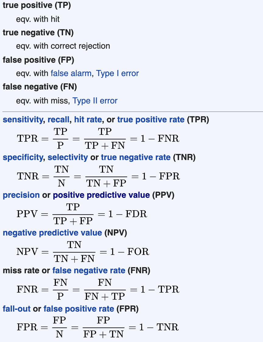
Confusion matrices

Names	Predict = 0	Predict = 1
Actual = 1	False Negative (FN)	True Positive (TP)
Actual = 0	True Negative (TN)	False Positive (FP)

confusion_on_logistic

Name	Alt Name	Formula
False Positive Rate	Type I error	$\frac{FP}{FP+TN}$
True Negative Rate	Specificity	$\frac{TN}{FP+TN} = \frac{TN}{N}$
True Positive Rate	Sensitivity, Recall	$\frac{TP}{TP+FN} = \frac{TP}{P}$
False Negative Rate	Type II error	$\frac{FN}{TP+FN}$
Precision		$\frac{TP}{TP + FP}$
Compiled measures
Overall Accuracy		$\frac{TP+TN}{FP + FN + TP + TN}$
ROC Curve	Plot TPR against FPR

Wikipedia reference

metrics-wikipedia

Evaluation Metrics

library(caret)
caret::confusionMatrix(as.factor(predictLog_train > 0.5),
                       as.factor(train$spam==1))


# please ensure correct order
CM = table(predictforest,test$rev)
CM
# predictforest  0  1
#             0 47 21
#             1 35 81
Accuracy = (CM[1,1]+CM[2,2])/sum(CM)
Accuracy # 0.6956522 vs 0.7119565
BaseAccuracy =  (sum(CM[1:2,1]))/sum(CM)
BaseAccuracy # or flip it
Sensitivity = (CM[1,1])/sum(CM[1:2,1])
Sensitivity
Specificity = (CM[2,2])/sum(CM[1:2,2])
Specificity

Recevier Operating Curve

Probably you should write an analysis procedure given predicted probs and actual binary.

library(ROCR)
# even shorter function names are advisable
# but we can be explicit in this document
accuracy <- function(predict_object, data, threshold=0.5) {
  return(sum(diag(table(predict_object >= threshold, data))) /
           sum(table(predict_object >= threshold, data)))
}
auc <- function(predict_object, data) {
  prediction_obj <- prediction(predict_object, data)
  perf_obj <- performance(prediction_obj, measure = "auc")
  return(perf_obj@y.values[[1]])
}



library(ROCR)
# ROCR method to obtain predicted probs and actual labels
ROCRpred <- prediction(Pred[1:138],orings$Field[1:138])
# ROCR method to plot ROC curve
ROCRperf <- performance(ROCRpred,x.measure="fpr",measure="tpr")
plot(ROCRperf)  # simple plot
plot(ROCRperf,
     colorize=T,
     print.cutoffs.at=c(0,0.1,0.2,0.3,0.5,1),
     text.adj=c(-0.2,1.7))

# Calculate area under curve (AUC)
as.numeric(performance(ROCRpred,measure="auc")@y.values)

Predictive Models I

You will train a predictive model on training data, use the model to generate predictions on the test data (and check for accuracy if possible).

These model should have already been tested in the midterms and will not be tested in the finals.

All methods should have a prediction function. For classification models you need to specify whether you want the class (binary) or response (probability).

pred_1_p <- predict(tree_1_o_2, newdata = test_1, type = "class")

Linear regression

Week 2

Method	Linear Regression
Target	Number
Model	$y_i = \beta_0 + \beta_1 x_1 + \beta_2 x_2 + ... + \epsilon_i$
Loss	Mean square error
Quality of fit	R-square Adjusted R-square AIC
Examples	Wine prices and quality Baseball batting average
Comments	Choose only the statistically significant variables This cannot predict binary objectives./

# fitting linear model
model1  <- lm(LPRICE~VINT+HRAIN,
              data=winetrain)
summary(model1)
confint(model7, level=0.99)  # see confidence interval

# predicting values with model
pred <- predict(model1,
                newdata=winetest,
                type="response")  # not sure if correct

coef(model1)

Logistic Regression

Week 3

Method	Logistic Regression
Target	Binary
Model	$P(y_i = 1) = \dfrac{1}{1+e^{-(\beta_0 + \beta_1 x_1 + \beta_2 x_2 + ...+ \epsilon_i )}}$
Loss	$LL(\beta) \\ = \displaystyle \sum_{i=1}^n \sum_{k=1}^2 y_{ik} \log \left( P(y_{ik} = 1) \right)\\= \displaystyle \sum_{i=1}^n \sum_{k=1}^2 y_{ik} \log \left( \dfrac{e^{\beta' x_{ik}}} {\sum_{l=1}^k e^{\beta' x_{il}}} \right)$
Explanation	$x \log (x’)$, sum over $x=1$ and $x=0$ (elaborate)
Quality of fit	$AIC = -2LL(\hat{\beta}) + 2(p+1)$ Confusion matrix AUC-ROC
Examples	Space shuttle failures Risk of heart disease
Comment

# fitting logisitic model (family = binomial)
model3 <- glm(Field~Temp+Pres,
              data=orings,
              family=binomial)
summary(model3)

# predicting probabilities with model
Pred <- predict(model4,
                newdata=orings,
                type="response")

coef(model4)

Multinomial Logit

Week 4a

Method	Multinomial Logit
Target	n-choose-1
Model	$$P(y_{ik} = 1	{ \text{options} }) = \dfrac{e^{\beta’ x_{ik}}} {\sum_{l=1}^k e^{\beta’ x_{il}}}$$
Loss	$LL(\beta) \\ = \displaystyle \sum_{i=1}^n \sum_{k=1}^K z_{ik} \log(P(y_{ik} = 1)) \\ = \displaystyle \sum_{i=1}^n \sum_{k=1}^K z_{ik} \log \dfrac{e^{\beta' x_{ik}}} {\sum_{l=1}^k e^{\beta' x_{il}}}$
Explanation	$z_{ik}$ is the training option from the dataset which is binary. $x_{ik}$ is the characteristic of one training option considered. ($x_{il}$ is similar, but it includes the rest of the training option included in the choice). You are tasked to provide $\beta’$ that maximises the log-likelihood. The probability that option $k$ is chosen from a set of choices is $P(y_{ik} = 1)$, and this is a real number.
Quality of fit	Log-likelihood Confusion matrix Likelihood ratio index $=1-\frac{LL(\beta)}{LL(0)}$ AIC $=-2LL(\beta) + 2p$
Examples	Academy Award winners
Comment	Independence of Irrelevant Alternatives - adding in a third alternative does not change the ratio of probabilities of two existing choxwices. (Probably it still does affect the training process?)

# (on data with the multiple choices over different rows)
library("mlogit")
# extracting data
D1 <- mlogit.data(subset(oscarsPP, Year <=2006), 
                  choice="Ch", 
                  shape="long", 
                  alt.var = "Mode")

# fitting multinomial logistic model
MPP2 <- mlogit(Ch~Nom+Dir+GG+PGA-1, data=D1)

# predicting probabilities with model
D1_new <- mlogit.data(subset(oscarsPP, Year==2007), 
                      choice="Ch", 
                      shape="long", 
                      alt.var="Mode")
Predict2 <- predict(MPP2, newdata=D1_new)

# (on data with the multiple choices on one row)
library(mlogit)
# extracting data
S <- mlogit.data(subset(safety, Task<=12), 
                 shape="wide",  
                 # this is "wide"-form data, unlike Oscars
                 choice="Choice", 
                 varying=c(4:83), 
                 sep="", 
                 alt.levels=c("Ch1", "Ch2", "Ch3", "Ch4"),
                 id.var="Case")

# fitting multinomial logistic model
M <- mlogit(Choice~CC+GN+NS+BU+FA+LD+
            BZ+FC+FP+RP+PP+KA+SC+TS+NV+
            MA+LB+AF+HU+Price-1, 
            data=S)

# predicting probabilities with model 
# this is done on training data
# for test data, create a new mlogit.data with Task>12
P <- predict(M, newdata=S)

# constructing confusion matrix with predictions
ActualChoice <- subset(safety, Task<=12)[,"Choice"]
PredictedChoice <- apply(P,1,which.max)
Tabtrain=table(PredictedChoice, ActualChoice)
Tabtrain

The willingness to pay can be observed from the survey, even though we do not directly ask the customers’ valuation.

When the model is fitted, the price has a negative coefficient while the safety features usually have a positive coefficient.
The ratio of the coefficients is the price that customers on the average is willing the pay.
The deviation can be observed the from standard error.

Mixed Logit

Week 4b

Method	Mixed Logit
Target	n-choose-1
Model	$$P(y_{ik} = 1	{ \text{options} }) = ???$$
Loss	`???`
Quality of fit	Log-likelihood Confusion matrix Likelihood ratio index $=1-\frac{LL(\beta)}{LL(0)}$ AIC $=-2LL(\beta) + 2p$ (number of paramters is now double)
Prediction	Preference of safety features
Comment	The data structure of safety feature options is different from the Academy Award. (elaborate) You can also evaluate how much people will pay for a certain extra feature, without directly getting their evaluation. (explore)

Screen Shot 2019-10-14 at 03.23.48 AM

#(please prepare S, the mlogit.data as per 4a second part)

# fitting mixed logistic model
M1 <- mlogit(Choice~CC+GN+NS+BU+FA+LD+
             BZ+FC+FP+RP+PP+KA+SC+TS+NV+
             MA+LB+AF+HU+Price-1, 
             data=S,
             rpar=c(CC='n',GN='n',NS='n',BU='n',FA='n',
                    LD='n',BZ='n',FC='n',FP='n',RP='n',
                    PP='n',KA='n',SC='n',TS='n',NV='n',
                    MA='n',LB='n',AF='n',HU='n',Price='n'),
             panel = TRUE, 
             print.level=TRUE)
summary(M1)

# predicting probabilities with model (with training data)
P1 <- predict(M1, newdata=S)

# constructing confusion matrix with predictions
PredictedChoice1 <- apply(P1, 1, which.max)
ActualChoice <- subset(safety, Task<=12)[,"Choice"]
Tabtrainmixed = table(PredictedChoice1, ActualChoice)
Tabtrainmixed

“The mixed logit model does a better job of predicting customers who are not interested in choosing any of the offered options compared to MNL.”

Regsubset

Week 5a

Method	Linear Regression with Subset Selection
Target	Number
Model	$y_i = \beta_0 + \beta_1 x_1 + \beta_2 x_2 + ... + \epsilon_i$
Loss	Mean square error
Quality of fit	R-square Adjusted R-square AIC
Examples	Wine prices and quality Baseball batting average
Comments	Choose only the statistically significant variables This cannot predict binary objectives.

Feature selection, based on the adjusted R-value from linear regression.

# fitting linear model, exhaustive feature selection
model2 <- regsubsets(Salary~.,
                     hitters,
                     nvmax=19)

# fitting linear model, exhaustive feature selection
model3 <- regsubsets(Salary~.,
                     data=hitters,
                     nvmax=19,
                     method="forward")

# fitting linear model, exhaustive feature selection
model4 <- regsubsets(Salary~.,
                     data=hitters,
                     nvmax=19,
                     method="backward")

# getting the coefficient of the best model with n params 
which.max(summary(model3)$adjr2)
coef(model3,3)

# heat map showing the best-n selected variables
plot(model1,scale=c("adjr2"))

LASSO

Week 5b

Balance data fit (first term) with model complexity (second term) $\underset{\beta}{min} \sum_{i=1}^{n} (y_i - \beta_0 - \beta_1 x_{î} - ... - \beta_p + x_{ip})^2 + \lambda \sum_{j=1}^p |\beta_j|$ The objective coefficient in LASSO is convex and tries to roughly promote sparsity.

Advantage of LASSO is that since it is convex, the local optimum is the global optimum.

Unfortunately, objective function is not differentiable unlike standard linear regression. But there are efficient ways to solve the problem to optimality.

Following is ridge regression. The issue with ridge regression is that it does not promote sparsity (i.e. reduce the number of variables in the model).

\[\underset{\beta}{min} \sum_{i=1}^{n} (y_i - \beta_0 - \beta_1 x_{î} - ... - \beta_p + x_{ip})^2 + \lambda \sum_{j=1}^p \beta_j^2\]

Elastic Net combines both penalities.

Method	LASSO
Target	Number
Model	$y_i = \beta_0 + \beta_1 x_1 + \beta_2 x_2 + ... + \epsilon_i$
Loss	$\underset{\beta}{min} \sum_{i=1}^{n} (y_i - \beta_0 - \beta_1 x_{î} - ... - \beta_p + x_{ip})^2 + \lambda \sum_{j=1}^p$
Quality of fit	According to loss
Prediction	Hitters
Comments	Choose only the statistically significant variables This cannot predict binary objectives.

# loading the dataset
library(glmnet)
X <- model.matrix(Salary~.,hitters)
y <- hitters$Salary

# train-test split
train <- sample(1:nrow(X),nrow(X)/2)
test <- -train

# fitting the lasso model with a specified schedule
modellasso <- glmnet(X[train,],y[train],lambda=grid)

# fitting the lasso model with a automatic grid
modellasso <- glmnet(X[train,],y[train],lambda=grid)

# show the plot of model lasso (please interpret)
# shows the value of the coefficient against L1 norm
plot(modellasso)           # plot against L1 Norm
plot(model4,xvar="lambda") # plot against lambda
model4$beta !=0            # plot with characters

# prediction (what is the difference?)
predictlasso1 <- predict(modellasso,
                         newx=X[test,],
                         s=100) 
predictlasso1a <- predict(modellasso,
                          newx=X[test,],
                          s=100,
                          exact=T,
                          x=X[train,],
                          y=y[train])

# calculation of mean square error
mean((predictlasso1-y[test])^2)

# does k-fold cross-validation for glmnet, 
# produces a plot
# returns a value for lambda
cvlasso <- cv.glmnet(X[train,],y[train])

Predictive Models II

Models that will be tested in finals.

CART

Week 8

Method	Classification and Regression Trees
Target	Customisable
Model	?
Loss	Does not attempt to find global minimum
Quality of fit	?
Prediction	Supreme Court decision
Comments

library(rpart)
library(rpart.plot)


# fitting with CART
cart1 <- rpart(rev~petit+respon+circuit+lctdir+issue+unconst,
               data=train, 
               method="class")
# plot the tree
prp(cart1, type=4, extra=2)

Pruning the tree

# Display the cp table for model cart1
printcp(cart1)
# We can also plot the relation between cp and error
plotcp(cart1)
# printcp() gives the minimal cp for which the pruning happens.
# plotcp() plots against the geometric mean

# print number of splits
unname(tail(tree_1_e$cptable[,2], 1))

# pruning the tree based on complexity parameter
cart2 <- prune(cart1,cp=0.01)
fancyRpartPlot(cart2)
predictcart2 <- predict(cart2,newdata=test,type="class")
table(test$rev,predictcart2)

# predicting with CART
predictcart1_prob <- predict(cart1, newdata = test)
# AUC procedure
#pred_cart1 <- prediction(predictcart1[,2], test$rev)
#perf_cart1 <- performance(pred_cart1,
#                          x.measure="fpr",measure="tpr")
#plot(perf_cart1)
#as.numeric(performance(pred_cart1,measure="auc")@y.values)

# to understand the options of rpart
?rpart.control

As the optimisation for global minimum is not computationally feasible, we use a heuristic approach instead. $\underset{\{R\}}{\min} \sum_{m=1}^M \sum_{i \in R_m} (y_i - \hat{y}_{R_M})^2$

Start with all observations in one region.

Choose predictor and cut-point such that $\underset{\{p\}}{\min} \underset{S}{\min} \left[ \sum_{i: x_{is} \leq S} (y_i - \hat{y}_{R_1})^2 + \sum_{i: x_{is} > S} (y_i - \hat{y}_{R_1})^2 \right]$

or other metric of performance such as entropy.

Solve a sequence of locally optimal problems with exhaustive search. The cut point is one of the the data points, along one of the dimensions.

Repeat each branch iteratively. Exit the branch when one exit condition is met.

For example, each prescribed bucket of leaves reached the prescribed minimum size.

Note that all observations belong to a single sub-region beyond which greedy splits are made at each step without looking necessarily at the best split that might lead to a better tree in future steps (greedy strategy) - in other words, local optimum at each step may not provide the global optimum.

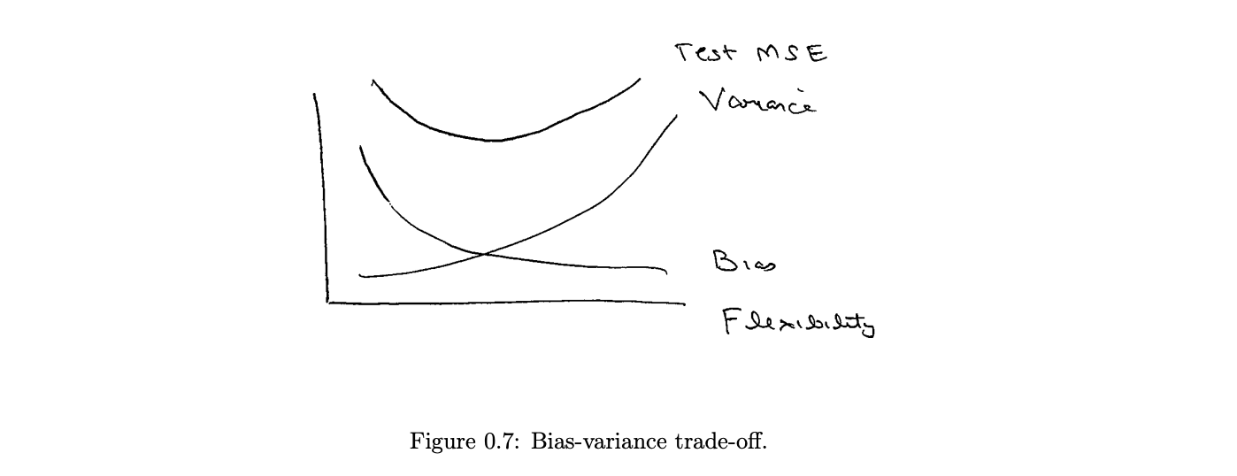
Bias variance trade-off

There is a trade-off between the model interpretability and performance on the training set.

To control the bias-variance trade-off (or, simply, the model complexity), CARTs use prepruning and pruning.

bias-variance-tradeoff

Breaking down the CART

When you print the model you get this guide

node), split, n, loss, yval, (yprob)
      * denotes terminal node

Following is the root node, with 434 points. If the leaf terminates here the absolute error is 195 points by predicting all 1s.

  1) root 434 195 1 (0.44930876 0.55069124)

After the first split (lctdir=liberal) there are 205 points that belongs to this split.

If the leaf terminates there, the absolute error is 82 points by predicting all 0s.

     2) lctdir=liberal 205  82 0 (0.60000000 0.40000000)

After the first split (lctdir=conser) there are 229 points that belongs to this split.

If the leaf terminates there, the absolute error is 72 points by predicting all 1s.

     3) lctdir=conser  229  72 1 (0.31441048 0.68558952)

Random Forests

Week 9

Method	Random Forests
Target	Customisable
Model	?
Loss	Customisable
Quality of fit	Customisable
Prediction	Social media
Comments	?

Intuition of ensemble training - each person have different knowledge, and different logical framework. Individual trees may not be accurate (and are faster to train), but make the ensembled prediction is more accurate. (Analogy - Who Wants to be a Millionaire)

Sample the training dataset with replacement (boosting or bagging)

Build a classification or regression tree
When splitting a node
Randomly choose $m$ parameters
Find the best cut-point by exhasutive search
Stop when the exit condition is met

Training a tree in a forest is faster than training a CART because only a subset of predictors are used.

Meta-parameters

The training does not optimise the meta-parameters.

$T^*$ number of tree in the ensemble ntree (recommended 100 to 1000)
$m$ = number of predictors chosen when creating a split mtry (recommended sqrt(p) for classification, p/r for regression)
$n_{min}$ minimum number of nodes in each leaf nodesize (recommended 2 to 20)

Downsides (compart to CART)

slower (though parallelizable across cores)
less interpretable

library(randomForest)

# set seed
#
# Build a forest of 200 trees, with leaves 5 observations in the terminal nodes

forest <- randomForest(as.factor(rev)~petit+respon+circuit+unconst+lctdir+issue, data=train, nodesize=5, ntree=200)
forest
# remember to convert the target variable into a factor

# The prediction is carried out through majority vote (across all trees)
predictforest <- predict(forest, newdata = test, type="class")
table(predictforest, test$rev)

Which of the variables is the most important in terms of the number of splits?

vu <- varUsed(rf_1, count = TRUE)
vusorted <- sort(vu, decreasing = FALSE, index.return = TRUE)
dotchart(vusorted$x, names(rf_1$forest$xlevel[vusorted$ix]))

Which of the following variables is the most important in terms of mean reduction in impurity?

varImpPlot(forest)
# forest$importance

Naive Bayes

Week 10

Method	Naive Bayes’
Target	Binary
Model	?
Loss	?
Quality of fit	?
Prediction	?
Comments	Based on a (naive) hypothesis of conditional independence of the features

Bayes Theorem $P(A|B) \cdot P(B) = P(B|A) \cdot P(A)$

We now make a (naive) hypothesis of conditional independence of the features, that is, $x_i$ is conditionally independent of every other feature $x_j$ (with $i \neq j$).

library(e1053)
# train the model
model3 <- naiveBayes(as.factor(responsive)~.,data=train)
summary(model3)

# ???
model3$apriori
# Y
# 0   1 
# 500  96 

# List tables for each predictor. For each numeric variable, it gives target class, mean and standard deviation.
model3$tables[5]

# predict with model
predict3 <- predict(model3,newdata=test,type="class")
table(predict3,test$responsive) 

naive-bayes-classifier

Collaborative Flitering

Week 10

Method	Collaborative Flitering
Target	Rating (regression)
Model	?
Loss	RSME $= \sqrt{\sum_{i=1}^u (r_{ui}-p_{ui})^2/u}$
Quality of fit	?
Prediction	Recommendation Systems
Comments	Objective of recommendation systems - accuracy, variety, updatable, computationally efficient

Essentially, take the average of the nearest 250 users, promixity is calculated by correleation.

Limitations

Inconsistent number of ratings given to each items
“Cold start” - struggles with new users

Instead of clustering by genres, we can predict a user’s rating on a movie, with all the past ratings done by all the users.

We can calculate the similarity across different users (we only calculate for the obects that has been rated by both users).

Baseline predictions for a movie by a user

take the average of the prediction on the movie
take the average of the prediction by the user

Predictive models

Identify the cluster that the test user was classified into
- Take the average rating by the cluster on the movie
- Take a weighted average taking into account of the relative importance of each user in the subcluster (not all people in the cluster has rated the novie.)
- Take into account bias of the user on movie - replace the average rating the user has been given with the average rating the subcluster gives.

Dataset processing

To decrease storage and transfer size, we are usually given list of ratings. Each rating consists of the rater (user) and the rated (movie), and the score.

length(unique(ratings$userId))  # 706
length(unique(ratings$movieId)) # 8552
sort(unique(ratings$rating))    # 0.5 1.0 ... 5.0

We need to transform this into a spare matrix for our input. We first create an empty matrix and them populate it.

Data <- matrix(nrow=length(unique(ratings$userId)), ncol=length(unique(ratings$movieId)))

for(i in 1:nrow(ratings)){
  Data[as.character(ratings$userId[i]),
       as.character(ratings$movieId[i])] <- ratings$rating[i]}

Train test split in a matrix

Type	Movies
Users	Training data	Data to make baseline prediction
	Data to make baseline prediction	Test set

# We want to create a matrix with 
# spl1 + spl1c rows and spl2 + spl2c columns

set.seed(1)       
spl1 <- sample(1:nrow(Data), 0.98*nrow(Data)) 
# spl1 has 98% of the rows
spl1c <- setdiff(1:nrow(Data),spl1)           
# spl1c has the remaining ones

set.seed(2)
spl2 <- sample(1:ncol(Data), 0.8*ncol(Data))  
# spl2 has 80% of the columns
spl2c <- setdiff(1:ncol(Data),spl2)           
# spl2c has the rest

# spl(s) are indices
length(spl1)  # 691
length(spl1c) # 15
length(spl2)  # 6841
length(spl2c) # 1711

We initialise the matrices to fill in our predictions. It should have the same dimension with our test set.

test_set <- Data[spl1c, spl2c]
Base1    <- matrix(nrow=length(spl1c), ncol=length(spl2c))
Base2    <- matrix(nrow=length(spl1c), ncol=length(spl2c))
UserPred <- matrix(nrow=length(spl1c), ncol=length(spl2c))

Baseline predictions

The predicted rating by each user on a movie is the average of all predictions on the movie. A movie will have the same prediction, by any user.

for(i in 1:length(spl1c))  
{Base1[i,] <- colMeans(Data[spl1,spl2c], na.rm=TRUE)}
Base1[,1:10] 
# All rows (users) contain the same information

The predicted rating by a user on each movie is the average of all predictions by the user. A user will provide the same rating for all movies.

for(j in 1:length(spl2c)) 
{Base2[,j] <- rowMeans(Data[spl1c,spl2], na.rm=TRUE)}
Base2[,1:10] 
# All columns (movies) contain the same information

Correlation model

Essentially, we are taking the average prediction of the nearest $N$ users. We first initialse a matrix to contain the correleation between each pair of users.

# Initialize matrices
Cor <- matrix(nrow=length(spl1),ncol=1) 
# keeps track of the correlation between users
Order <- matrix(nrow=length(spl1c), ncol=length(spl1)) 
# sort users in term of decreasing correlations

For each user, we calculate the correlation with all other users. Then each user will have a list of all (or most due to NAs) other user, ordered with decreasing correlation.

# The NAs account for users who have no common ratings of movies with the user.
for(i in 1:length(spl1c)){
  for(j in 1:length(spl1)){
      Cor[j] <- cor(Data[spl1c[i],spl2],
                    Data[spl1[j],spl2],
                    use = "pairwise.complete.obs")
      }
  V <- order(Cor, decreasing=TRUE, na.last=NA)
  Order[i,] <- c(V, rep(NA, times=length(spl1)-length(V)))
}

The prediction of the user on a movie will be average of the nearest $N$ users. $N$ is a hyperparameter chosen by us.

# Now, we compute user predictions by looking at the 250 nearest neighbours and averaging equally over all these user ratings in the items in spl2c
for(i in 1:length(spl1c))
{UserPred[i,] <- colMeans(Data[spl1[Order[i,1:250]],spl2c], na.rm=TRUE)}    
UserPred[,1:10]

Compare the model performance

We take the average of the squared difference with the test set.

RMSEBase1    <- sqrt(mean((Base1 - test_set)^2, na.rm=TRUE))
RMSEBase2    <- sqrt(mean((Base2 - test_set)^2, na.rm=TRUE))
RMSEUserPred <- sqrt(mean((UserPred - test_set)^2, na.rm=TRUE))


# Last step: we vary the neighborhood set for the third model to see whether it positively affects the results
RMSE <- rep(NA, times=490)
for(k in 10:499)
{for(i in 1:length(spl1c))
  {UserPred[i,] <- colMeans(Data[spl1[Order[i,1:k]],spl2c], na.rm=TRUE)}
  RMSE[k-10] <- sqrt(mean((UserPred - test_set)^2, na.rm=TRUE))}
plot(10:499,RMSE)

Each user is represented through a vector of items (e.g. movie) and the associated rating given to each itme.

Inconsistent number of rating across items

Each items is represented by a vector of attributes.

Tobit model

Week 11

Method	Tobit model
Target	Number
Model	?
Loss	?
Quality of fit	?
Prediction	?
Comments	For left or right censored data

library(survival)
# the Tobit model
model1 <- survreg(Surv(time_in_affairs,
                       time_in_affairs>0,type="left")~.,
                  data=train, dist="gaussian")
summary(model1)
predict1 <- predict(model1,newdata=test) 
table(predict1<=0,test$time_in_affairs<=0)

# using linear model as baseline
model2 <- lm(time_in_affairs~., data=train)
summary(model2)
predict2 <- predict(model2,newdata=test)
table(predict2 <= 0, test$time_in_affairs==0)

This applies to censored target, does this apply to censored parameters as well?

Non-predictive models

These are models that do not produce a prediction. The output, however, can be used as a feature to the predictive models.

Supervised learning versus unsupervised learning Supervised learning. Given a set of predictors ${x_1, …, x_p}$ and an output of ${y}$, we want to find a function $f(x_1, …, x_p) = \hat{y}$ that minimise the error on some metric.

Unsupervised learning. Given a set of features, we want to find “patterns” within the data. Find a group of clusters that minimise the intra-cluster variance and maxisies the inter-cluter vairance.

K-means clustering

Week 10

Method	K-means clustering
Target	Clusters
Model	?
Loss	?
Quality of fit	?
Prediction	Recommendation Systems
Comments	?

Algorithmic Procedure

Initialisation - Given a number of clusters $k$, randomly generate $k$ different means/centroids.

Assign each observation to the cluster whose mean/centroid has the closest Eculidean distance.

Update calculate the new means/centroid, and repeat assignment.

Stop when the assignment does not change.

Downsides

May end up with different results
May not converge or take a very long time to converge.

# execute k-means clustering
# n-start is the number of different starting points
# choose the best clustering from each of the n-start
clusterMovies2 <- kmeans(Data[,1:19], centers=10, nstart=20)

# the loss within each cluster
clusterMovies3$withinss

# the total loss for all the clusters
clusterMovies2$tot.withinss # 7324.78

# Plot loss against k
fit <- c()
for(k in 1:15){
  clusterMovies4 <- kmeans(Data[,1:19], centers=k, nstart=20);
  fit[k] <- clusterMovies4$tot.withinss}
plot(1:15,fit)

# calculate the average of each feature in the cluster
Cat2 <- matrix(0,nrow=19,ncol=10)
for(i in 1:19){
  Cat2[i,] <- tapply(Data[,i], clusterMovies2$cluster, mean)}
rownames(Cat2) <- colnames(Data)[1:19]
Cat2

# list the elements in the cluster
subset(Data$title, clusterMovies2$cluster==6)

Hierarchical clustering

Week 10

Method	Hierarchical clustering
Target	Dendrogram, Clusters
Model	?
Loss	?
Quality of fit	?
Prediction	Recommendation Systems
Comments	?

Algorithmic Procedure

Compute the Euclidean distance between each pair. The closest pair forms a cluster and we take the midpoint. The output is a dendrogram (which is a binary tree).

In the visualisation, the distance of the vertical edge represents the distance between adjacent leaves. The horizontal placement and distance do not have a meaning. Unlike K-means clustering, there is no need for any hyperparamter tuning to build a dendrogram.

To create a cluster, we need to select a cutoff distance. Each tree cut by the cutoff is one cluster each. A cluster may only have one leaf, we can this an atomic cluster.

One reason not to use hierarchical clustering - We might have too many observations in the dataset for hierarchical clustering to handle.

You need to do preprocessing to convert the list of genre for each movie into to a binary list.

# compute the distance between every pair
distances <- dist(Data[,1:19], method="euclidean")
dim(Data)
length(distances)

# execute hierarchical clustering 
# Ward's distance method is used to find compact clusters.
clusterMovies1 <- hclust(distances, method="ward.D2")

# plot dendrogram
plot(clusterMovies1) 

# create 10 clusters (by what criteria? binary search for cutoff?)
clusterGroups1 <- cutree(clusterMovies1, k=10)

# calculate the average of each feature in the cluster
Cat1 <- matrix(0,nrow=19,ncol=10)
for(i in 1:19){
  Cat1[i,] <- tapply(Data[,i], clusterGroups1, mean)}
rownames(Cat1) <- colnames(Data)[1:19]
Cat1

# list the elements in the cluster
subset(Data$title, clusterGroups1==6)

Text mining

Converts text into number for predictive models.

Read the dataset. Each entry of the dataset is a ‘document’. A corpus is a set of documents

library(tm)
library(SnowballC)
library(wordcloud)

twitter <- read.csv("wk9a-text.csv",stringsAsFactors=FALSE)
corpus <- Corpus(VectorSource(twitter$tweet))

Conduct text transformations to simplify the dataset.

# list of text transfomrations
getTransformations()

# transformation into lower case
corpus <- tm_map(corpus, function(x) iconv(enc2utf8(x), sub = "byte"))
corpus <- tm_map(corpus, content_transformer(function(x) iconv(enc2utf8(x), sub = "bytes")))
corpus <- tm_map(corpus,content_transformer(tolower))

# remove stop words
corpus <- tm_map(corpus,removeWords,
stopwords("english"))
                                            
# remove specific words because they confuse the objective
corpus <- tm_map(corpus,removeWords,
c("drive","driving","driver","self-driving","car","cars"))  

# remove punctuation 
corpus <- tm_map(corpus,removePunctuation)

# stemming words (get root word)
corpus <- tm_map(corpus,stemDocument)

Convert into a document term matrix. This is a freqlist of every document in the corpus.

# convert into freqlist of words this will be a sparse matrix
dtm <- DocumentTermMatrix(corpus)
dim(dtm) # dimensions before removal
dtm <- removeSparseTerms(dtm,0.995)

Transforming into a dataframe to train and test

# converting DTM into dataframe                                            
twittersparse <- as.data.frame(as.matrix(dtm))

# make sure column names start with a character
colnames(twittersparse) <- make.names(colnames(twittersparse))

# assign labels to dataframe                                            
twittersparse$Neg <- twitter$Neg

Visualise the dataset with a wordcloud.

# plot wordcloud                                
colnames(twittersparse) <- make.names(colnames(twittersparse))
colnames(twittersparse)
word_freqs = sort(colSums(twittersparse), decreasing=TRUE) 
# Create dataframe with words and their frequencies
dm = data.frame(word=names(word_freqs), freq=unname(word_freqs))
# Plot wordcloud
wordcloud(dm$word, dm$freq, random.order=FALSE, max.words=100, colors=brewer.pal(8, "Dark2"), min.freq=2)

Then carry out your model based on their mdoels.

Singular Value Decomposition

Week 11

Method	Singular Value Decomposition
Target	?
Model	?
Loss	?
Quality of fit	?
Prediction	NA
Comments	For image compression

Review of linear algebra

# define a matrix
A <- matrix(c(2, 2, 3, 1), nrow=2, ncol=2)

# Get eigenvectors and eigenvalues
A_eig <- eigen(A)
A_eig$values
A_eig$vectors # these vectors are normalised

Eigen decomposition $A = V \cdot S \cdot V^{-1}$

$V$ is a square matrix made up of columns of eigenvectors, and $S$ is a square matrix with its main diagonal made up of eigenvalues is the corresponding order.

# reconstruct the matrix
# (note the operator %*% for the matrix multiplication)
A_eig$vectors %*% diag(A_eig$values) %*% solve(A_eig$vectors)

If $A$ is positive semi definite (eigenvalues of A is non-negative), $V^{-1} = V^T$

Singular Value Decomposition $\underset{m \times n}{X} = \underset{m \times n}{U} \cdot \underset{n \times n}{S} \cdot \underset{n \times n}{V^{T}}$

It can be shown that

\[X \cdot X^T = U \cdot S^2 U^T\] \[X^T \cdot X = V \cdot S^2 V^T\]

$U$ contains the $m$ eigenvectors of $X \cdot X^T$ (left singular vectors)

$S$ contains the $n$ square roots of $X \cdot X^T$ eigenvalues (singular values)

$V$ contains the $n$ eigenvectors of $X^{T} \cdot X$ (right singular vectors)

X <- matrix(c(2,1,5,7,0,0,6,0,0,10,
              8,0,7,8,0,6,1,4,5,0), nrow=5, ncol=4)

s <- svd(X) # apply SVD
s$u # U
s$d # S
s$v # V

# reconstruct the matrix
s$u %*% diag(s$d) %*% t(s$v)

When R implements SVD it transforms it into $m > n$. Check the function parameters of svd() for variations.

Approximating a matrix $\underset{m \times n}{\hat{X}} = \underset{m \times k}{U_k} \cdot \underset{k \times k}{S_k} \cdot \underset{k \times n}{V_k^{T}}$

# reconstruct a matrix with limited elements
k <- 2  # less than or equal to n
s$u[,1:k] %*% diag(s$d[1:k]) %*% t(s$v[,1:k])

Calculate explained variance Frobenius norm of a matrix $||x||_F$ $||X||_F = \sqrt{\sum_{i=1}^m \sum_{j=1}^n x_{i,j}^2}$

\[\frac{||\hat{X}||_F}{||X||_F} = \frac{\sigma_1^2 + ... + \sigma_k^2} {\sigma_1^2 + \sigma_1^2 + ... + \sigma_n^2}\]

# calculate the explained variance
var <- cumsum(s$d^2)
plot(1:4,var/max(var))

Image compression with SVD

For grayscale images

# read image
lky <- readJPEG("wk11-gray.jpg")

# grayscale images has same values for all channels
# apply SVD on the image
s <- svd(lky[,,1])

# compress and save the image
k = 10
lky10 <- s$u[,1:k] %*% diag(s$d[1:k]) %*% t(s$v[,1:k]) 

# write image to file
writeJPEG(lky10,"wk11-gray10.jpg")

# calculate the explained variance
var <- cumsum(s$d^2)
plot(1:4,var/max(var))

For colored images

# read image
pansy <- readJPEG("wk11-color.jpg")

# apply SVD on the image
s1 <- svd(pansy[,,1])
s2 <- svd(pansy[,,2])
s3 <- svd(pansy[,,3])

# compress and save the image
k = 50
pansy50 <- array(dim=dim(pansy))
pansy50[,,1] <- s1$u[,1:k] %*% diag(s1$d[1:k]) %*% t(s1$v[,1:k])
pansy50[,,2] <- s2$u[,1:k] %*% diag(s2$d[1:k]) %*% t(s2$v[,1:k])
pansy50[,,3] <- s3$u[,1:k] %*% diag(s3$d[1:k]) %*% t(s3$v[,1:k])

# write image to file
writeJPEG(pansy50,"wk11-color50.jpg")

Kaplan-Meier estimator

Not a prediction model, estimate the chances of “occurance” over time just by the results.

An event will happen at a distribution with pdf $f(x)$ and corresponding cdf $F(x)$.

The hazard function is the instantaneous rate of probability the event happening $\lambda(t) = \frac{f(t)}{1-F(t)} = \frac{f(t)}{S(t)}$ Given the data, you can estimate $S(t) = 1 - F(t)$. $\hat{S}(t) = \prod_{t_i < t} \frac{n_i-d_i}{n_i}$ $n_i$ is the number of people who have survived until before $t_i$. If $t_i$ are continuous values, $d_i$ will always be one.

km <- survfit(Surv(start,stop,event)~1,data=heart)
summary(km,censored=TRUE) 
# summary of the model, with patients' survival probability 

# plot the Kaplan-Meier curve along with 95% confidence interval
plot(km) 

Cox proportional hazard model

This is a prediction model but I put it here. This estimate the chances of occurance over time, now taking into account of some parameters.

Week 11

Method	Cox proportional hazard model
Target	?
Model	$\lambda(t) = \lambda_0(t) \cdot e^{\beta_1 x_1 + \beta_2 x_2 + …}$
Loss	?
Quality of fit	?
Prediction	This is a linear model, with censored values.
Comments	?

An event will happen at a distribution with pdf $f(x)$ and corresponding cdf $F(x)$.

\[\lambda(t) = \lambda_0 \cdot exp(\beta_1 x_1 + ... + \beta)\]

cox <- coxph(Surv(start,stop,event)~age+surgery+transplant,
             data=heart)
summary(cox)
        
# plot S(t)
plot(survfit(cox))
summary(survfit(cox))

predict(cox, data=heart)