notes

Manufacturing and Service Operations

Instructors: Shruti and Lingjie

• Manufacturing and Service Operations
  • Course Overview
  • Inventory Management
    • News Vendor model
    • Base-stock model
    • Economic Order Quantity model
    • Economic Production Quantity Model
    • (Q,r) model
  • Discrete Time Markov Chains
    • Modeling A System As A DTMC
      • Chapman-Kolmogorov Equation
    • Reducible and Irreducible DTMC
    • Periodic and aperiodic DTMC
    • Recurrent and transient DTMC
    • Limiting Behavior of DTMC
    • Average cost models
  • Continuous Time Markov Chains
    • Mathmatical formulas
    • Some theorems of CTMC
    • Modeling A System As A DTMC
    • Steady state analysis
    • Cut analysis
    • Retrial queue
    • Average cost analysis

Course Overview

Component	Weightage (%)
Class Participation	5
Homework/Activities	20
Group Project	25
Midterms (Simulation)	25
Finals	25

Group project

• Choose either inventory or service management
• Ideally, work with a company on a relevant task
• You may resort to using public data

Inventory Management

Permutations of manufacturing operations

• Refer to week one notes, please make sure you can understand how each category is different.
• Periodic review versus continuous review
• Little’s Law
  • Average inventory / Average time = Average rate

Review of Excel functions

• NORMSDIST - the cumulative distribution function $\Phi(x)$ for standard normal distribution
• NORMSINV - inverse of the standard normal CDF
• PHI - probability density function $\phi(x)$ for a standard normal distribution
• NORMDIST(x,mean,standard_dev,cumulative)
  • x - The value for which you want the distribution.
  • mean - The arithmetic mean of the distribution.
  • standard_dev - The standard deviation of the distribution.
  • cumulative - TRUE or FALSE
    • If TRUE, NORMDIST returns the cumulative distribution function
    • if FALSE, it returns the probability density function.

For each model

• Variables and constants
• Assumptions
• Decision variable (What is being decided and optimised)
• Optimal condition
• Performance measures

• Identities (Not just for the optimal quantity)

• Miscellaneous

News Vendor model

This is periodic review

Variables and constants

• Demand of the period
  • with known continuous probability distribution $g(x)$ or $G(x)$
  • that has mean $\theta$ and standard deviation $\sigma$
• Overage cost $c_o$
• Shortage cost $c_s$ (which is also unit profit)

Assumptions

• Planning is done for a single period
• Deliveries are made in advance of demand
• No fixed cost (you are making a purchase at the start of each period anyway)
• Products can analysed individually - either a single product or no interactions between products

Decison variable

• $Q$ Order / production quantity (product units)

Opitimal order quantity $Q^*$

• $G(Q^*) = \dfrac{c_s}{c_o + c_s}$
• Where incremental overage cost exceed incremental shortage cost

Performance measures (for a certain order quantity $Q$)

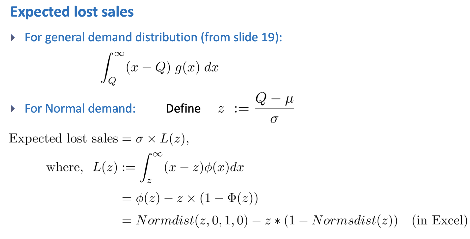
• Expected lost sales (units)
  • calculated based on the demand distribution and $Q$
  • 
• Expected demand (units)
  • $\mu$ of the given assumed distribution
• Expected sales (units)
  • expected demand $\mu$ $-$ expected lost sales
• Expected leftover inventory (units)
  • $Q$ the chosen supply $-$ expected sales
• Expected profit (dollars)
  • expected sales $\times$ shortage cost $–$ expected leftover inventory $\times$ overage cost
• Probability of shortage or overage
  • read from the probability distribution for demand

Identities (for all $Q$)

• Specified supply $Q$ $=$ Expected sales $+$ Expected leftover inventory
• Expected demand $\mu$ $=$ Expected sales $+$ Expected lost sales

News Vendor Model with Risk pooling

• Why not we use blanks to fulfill unmet demand of star player Jerseys?
  • If there is shortage, we can print using the blank
  • Printing in the US is still more expensive, so there is tradeoff
• Differences
  • Cost of overage is the same (could only salvage)
  • Cost of shortage is different
    • depends if blank is available
    • whether is it available is a probability (previously calculated)
      • for each of the two scenario there is a cost
    • this is an approximate
• Are we now only ordering blanks from the CM?
  • No, but less

How is the profit calculated? Example?

Base-stock model

This is continuous review.

Variables and constants

• Lead time $l$ (or replenishment time, fixed and known)
• Demand during replenishment lead time
  • with known continuous probability distribution $g(x)$ or $G(x)$
  • that has mean $\theta$ and standard deviation $\sigma$
  • (demand still happens one at a time)
• Unit holding cost $h$ (per unit, per time)
• Unit backorder cost $b$ (per unit, per time)

Assumptions

• Demand occurs one at a time, with i.i.d. interarrival times
• Replenishment units are ordered one at a time
• Unsatisfied demand is backordered, and will be fulfilled.
• No fixed cost. (The order is placed one at a time anyways)
• Products can analysed individually - either a single product or no interactions between products
• Initial amount of inventory is $r+1$

Decision variable

• Reorder point $r$
  • $r+1$ is the base-stock level

Optimal base-stock level $r^*+1$

• $G(r^*+1) = \dfrac{b}{h+b}$
• Where incremental holding cost exceed incremental backorder cost

Performance measures (for a certain reorder point $r$)

• Safety stock level $r - \theta$
• Expected backorder level
  • $B(r+1) = \int_{r+1}^{\infty} \enspace (x-r-1) \enspace g(x) \enspace dx$
  • If demand is normal
    • $(\theta -r -1)\left( 1 - \Phi \left[ \dfrac{r+1 - \theta}{\sigma} \right] \right) + \sigma \phi \left[\dfrac{r+1-\theta}{\sigma}\right]$
• Expected inventory level
  • (identity) $r+1 - \theta +$ Expected backorder level
  • Current inventory position = on-hand inventory + orders - backorders (Because negative inventory level is considered zero inventory)
• Fill rate
  • Fraction of demand satisfied instantaneously from on-hand inventory
  • $P (X \leq r+1) = P \left( \dfrac{X - \theta}{\sigma} \leq \dfrac{r+1-\theta}{\sigma} \right)$

Identities for all $r$

• Expected inventory level per unit time + Expected lead time demand = Expected number of backorders per unit time + Reorder point + 1

Model design

• Why r-plus-one?
  • This is so that $r$ is the reorder point, which can be zero.

Questions

• What happens if you have have a fixed cost of ordering?

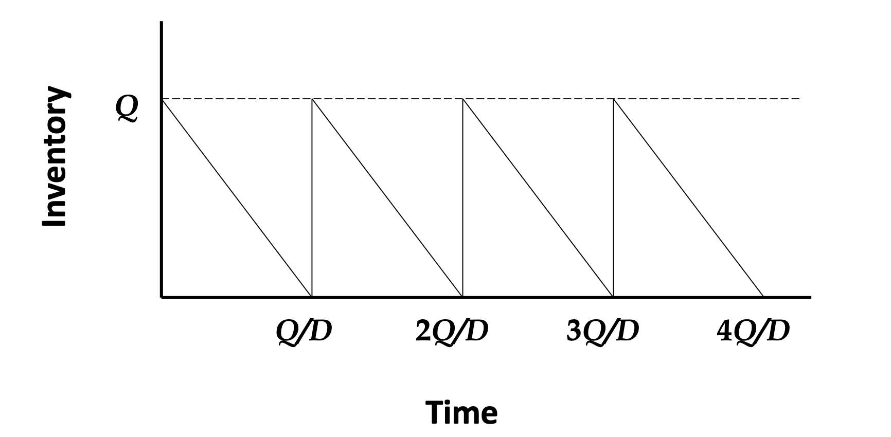
Economic Order Quantity model

This is continuous review (there is nothing to review actually, the setup is deterministic)

Variables and constants

• Demand rate $D$
• Fixed cost to place an order $A$
• Unit purchase/production cost $c$
• Unit holding cost $h$

Assumptions

• Unlimited rate of production capacity
• Instantaneous satisfaction of demand and no supply lead time
• Fixed setup cost to start production
• Products can analysed individually - either a single product or no interactions between products

Decision variable

• $Q$ The size of an order

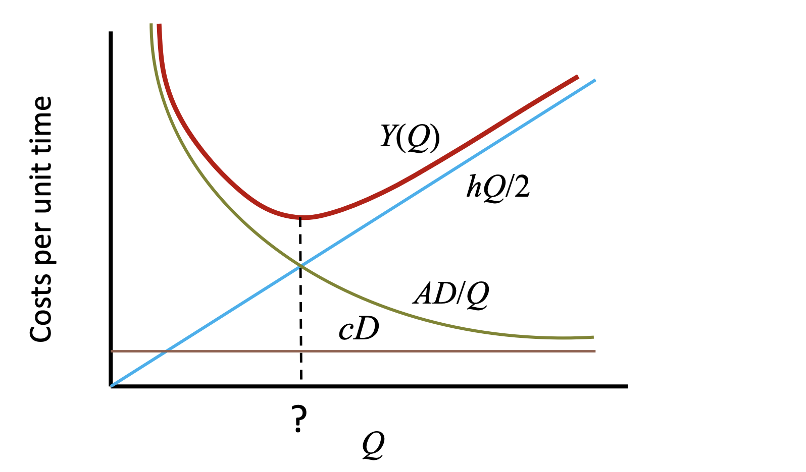
Optimal order quantity $Q^*$

• $Q^* = \sqrt{\dfrac{2AD}{h}}$
• Where incremental holding cost exceed decremental fixed order cost

Performance measures

• Total cost per unit time
  • $Y(Q) = \dfrac{hQ}{2} + \dfrac{AD}{Q} + cD$
• Total cost per unit time per unit product (not incremental)
  • $Y’(Q) = \dfrac{hQ}{2D} + \dfrac{A}{Q} + c$
• Average inventory
  • $\dfrac{Q}{2}$

Extension of EOQ

• Non-zero supply lead times
  • You will just order $L$ in advance
  • $Q^*$ is unchanged
• Non-zero safety stocks
  • Only a constant (holding cost) is added to the total cost
  • $Q^*$ is unchanged
• Finite production capacity
  • Economic Production Quantity Model

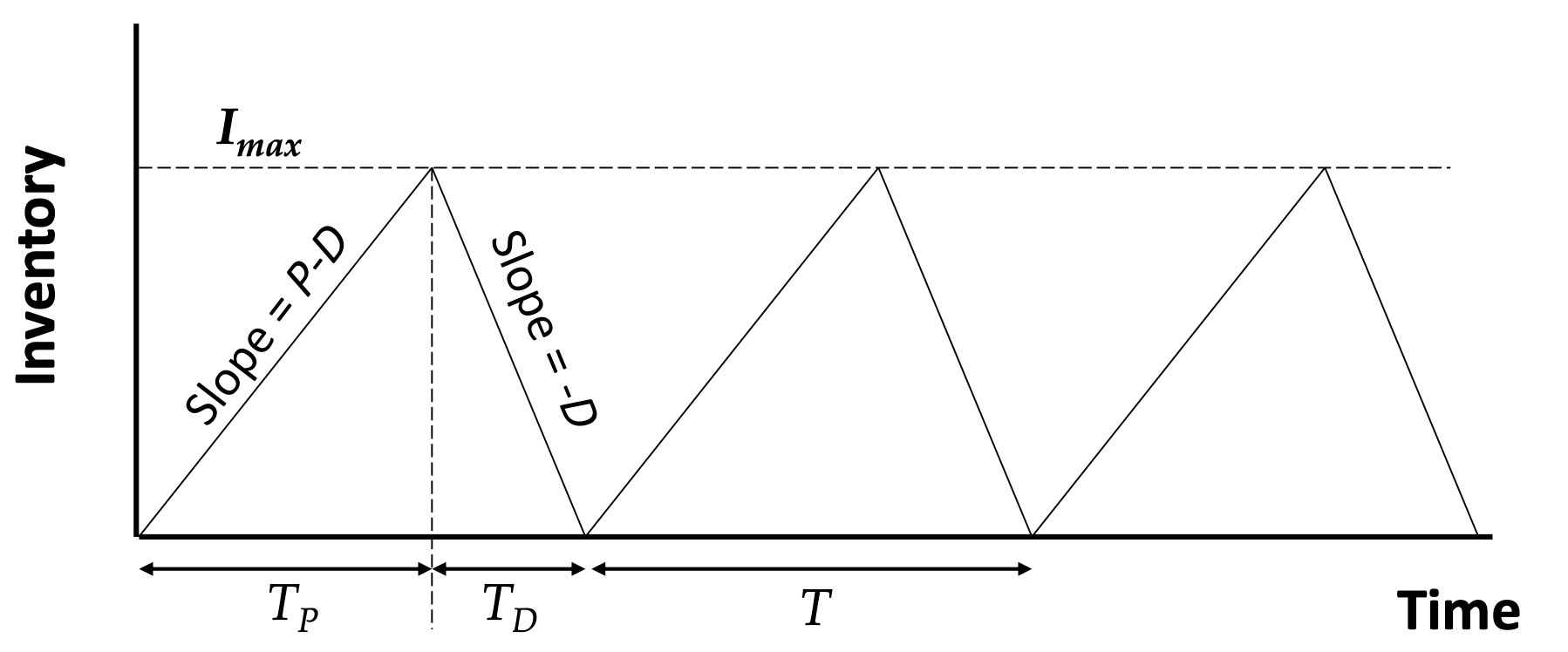
Economic Production Quantity Model

This is continuous review (there is nothing to review actually, the setup is deterministic)

The same as EOQ, except that production takes time.

Variables and constants

• Demand rate $D$
• Production rate $P$ (additional parameter from EOQ)
• Fixed cost to place an order $A$
• Unit purchase/production cost $c$
• Unit holding cost $h$

Assumptions

• Limited rate of production
• Determinisitic and constant demand which must be fulfilled
• Instantaneous satisfaction of demand and no supply lead time
• Fixed setup cost to start production
• Products can analysed individually - either a single product or no interactions between products

Decision variable

• $Q$ The size of an order

Optimal order quantity $Q^*$

• $Q^* = \sqrt{2ADh\left(1-\dfrac{D}{P}\right)} + cD$
• Where incremental holding cost exceed decremental fixed order cost

Performance measures (for a certain order quantity $Q$)

• Total cost per unit time
  • $Y(Q) = \dfrac{hQ}{2}\left(1-\dfrac{D}{P}\right) + \dfrac{AD}{Q} + cD$
• Total cost per unit time per unit product (not incremental)
  • $Y’(Q) = \dfrac{hQ}{2D}\left(1-\dfrac{D}{P}\right) + \dfrac{A}{Q} + c$
• Average inventory
  • $\dfrac{Q}{2} \left( 1 - \dfrac{D}{P} \right)$

(Q,r) model

This is continuous review.

Variables and constants

• Demand
  • with known continuous probability distribution $g(x)$ or $G(x)$
  • that has mean $\theta$ and standard deviation $\sigma$
  • (demand still happens one at a time)
• Fixed cost $A$ is associated with placing an order
• Fixed and known replenishment lead time $l$
• Unit purchase/production cost $c$ (per unit)
• Unit holding cost $h$ (per unit, per time)
• Unit backorder cost $b$ (per unit, per time)

Assumptions

• Unstatisifed demand is backordered
• Products can analysed individually - either a single product or no interactions between products

Decision variable

• $Q$ replenishment quantity
• $r$ the reorder point stock

Optimal decision variables

• $Q^* = \sqrt{\dfrac{2AD}{h}}$
  • Where marginal fixed order costs exceeds marginal holding costs
• $G(r^*) = \dfrac{b}{b+h}$
  • Where marginal holding cost exceeds marginal backorder costs

Performance measures

• Safety stock level $s= r - \theta$
• Expected backorder level
  • $B(Q,r) = \frac{1}{Q} \int_r^{r+Q} B(x) dx \lessapprox B(r)$
    • The appoximation is allowed as $\int_{r+Q}^{\infty} B(x) dx \gtrapprox 0 $
  • If demand is normal
  • $B(r) = (\theta - r)\left(1 - \Phi \left[ \dfrac{r-\theta}{\sigma} \right] \right) + \sigma \phi \left[ \dfrac{r-\theta}{\sigma} \right]$
• Expected inventory level
  • $I(Q,r) = \frac{1}{Q} \int_r^{r+Q} I(x) dx \ = \dfrac{Q}{2} + r - \theta + B(Q,r)$
• Fill rate
  • $S(Q,r) = \dfrac{1}{Q} \int_r^{r+Q} G(x) dx \ = 1 - \frac{1}{Q}[B(r) - B(r+Q)] \ \gtrapprox G(r) = \Phi \left[ \dfrac{r - \theta}{\sigma} \right] $
• Expected total cost
  • $Y(Q,r) = A \cdot F(Q,r) + h \cdot I(Q,r) + b \cdot B(Q,r)$

Identities for all $r$ and $Q$

• Inventory position = On-hand inventory + outstanding orders – backorders
  • Please understand which is which
• Inventory position is uniformly distributed between $r$ and $r+Q$

(Dark green - on-hand inventory, Red - negative of backorder, Orange - outstanding orders, Blue - inventory position)

Discrete Time Markov Chains

A special stochastic process satisfying “Markov/memoryless” (given previous state, the future is independent of the past) & “time-invariant”.

Modeling A System As A DTMC

• Determine $X_n$ the state of the system at the n-th observation.
• Write down the state space $\mathcal{S}$, i.e. the set values $X_n$.
• Check if memoryless and time-invariant properties hold in the modeling.
  • If yes, HURRAY!
  • If no, redefine ${X_n, n \geq 0 }$.
• Obtain the transition probability matrix $P$ (and transition diagram). Rows of $P$ should add up to one.

Advice

Draw the transition diagram. Outgoing arrows should add up to one.

Chapman-Kolmogorov Equation

\[[P^k]_{ij} = \sum_{r \in \mathcal{S}} [P^{k-l}]_{rj} [P^l]_{ir}\]

This is because of the time-invariant property.

Reducible and Irreducible DTMC

If it is possible to go from any state $i$ to any state $j$ with at least $k$ step, the DTMC is irreducible with $k$ steps.

Otherwise the DTMC is reducible.

Periodic and aperiodic DTMC

For any state if the probability of revisiting the state is non-zero after $d, 2d, 3d, \cdots$ steps.

A DTMC is aperiodic if $[P]_{ii} > 0$ for some state $i \in \mathcal{S}$ or $d=1$.

Recurrent and transient DTMC

Recurrent: If each state will be revisited sooner or later, the DTMC is recurrent.

Positive recurrent: the expected time to revisit any state is finite.

Null recurrent: If the DTMC is recurrent but not positive recurrent

Transient: If the DTMC is not recurrent.

Theroems

• For a finite-state DTMC, irreducible property guarantess recurrent.
• For a finite-state DTMC, all recurrent matrices are positive recurrent.

Limiting Behavior of DTMC

$\pi = a P^{\infty}$

If row vector $\pi$ exists, it is the stationary probability of the DTMC. $a$ is the initial row vector.

If the DTMC is apreiodic, the rows $P^{\infty}$ is made up of is equal to $\pi$.

Theorems

• A finite-state irreducible aperiodic DTMC has a unique $\pi$.
• A DTMC that is poth positive recurrent and aperiodic has a unique $\pi$. The DTMC is said to be ergodic.

Average cost models

A cost $C_i$ is incurred for observing state $i$.

The long-run average cost is

$C = \sum_{i \in \mathcal{S}} \pi_i C_i$

Continuous Time Markov Chains

The state can now change at any time.

Mathmatical formulas

Geometric progression

Sum to infinity

$\displaystyle\sum_{k=0}^\infty ar^k = \dfrac{a}{1-r}$

Sum of first n terms

$\displaystyle\sum_{k=0}^n ar^k = \dfrac{a(1-r^{n+1})}{1-r}$

Power identity (for full list refer to MF15 or search on Google)

$1 + 2 \rho + 3 \rho^2 + 4 \rho^3 + \cdots = \dfrac{1}{(1-p)^2}$

Some theorems of CTMC

Modeling A System As A DTMC

• Define $X(t)$, the state of the system at time $t$
• Write down $\mathcal{S}$, the state space.
• Obtain the generator matrix $Q$ and draw the rate diagram.

Steady state analysis

Cut analysis

Flow in mean rate = flow out mean rate

Rate = $\lambda_{ij} \cdot \pi_i$

Where $\lambda_{ij}$ is the transition rate of state $i$ to state $j$, and $\pi_i$ is the long term probability of the state $i$.

Strategy

• Express all $\pi_i$ everything in terms of $\pi_0$
  • Start the cut analysis from state 0
• Equate $\sum \pi = 1$ to solve for $\pi_0$
• Substitute $\pi_0$ into your expressions of $\pi_i$

Retrial queue

• $\lambda$ is the rate of passengers entering
• $\mu$ is the rate of passengers getting served
• $\theta$ is the rate of passengers in orbit starts to get served

How is this different from the normal queue

• The customers in the queue do not immediate get served when the server is idle.

After formulation

$\pi_{0,0} = \left[ (1-\dfrac{\lambda}{\mu})^{\frac{\lambda}{\mu} + 1} \right]$

Average cost analysis

The long run average cost per unit time is

$\sum_{i=0}^k C_i \pi_i$